One of Excels most powerful but sometimes overlook tools is the LOOKUP family of functions. While there are several variations, LOOKUP or HLOOKUP, learning how to use VLOOKUP in Excel has been a game-changer. Excel VLOOKUP allows you to quickly match and group data based on information stored elsewhere.
Why would I use a Vlookup
Firstly, let’s start with a basic example, a list of sales deals that have been closed this quarter. The list includes customer name, salesperson, and also total invoice amount. Each salesperson is assigned to a different region. So if I want to determine the total sales for a region I need to somehow group the data. I could go through and label each transaction with a region. Rather I can use VLOOKUP to assign a region based on the sales reps name.
What makes up the VLOOKUP Function?
= VLOOKUP (lookup_value, table_array, col_index_num, [range_lookup])
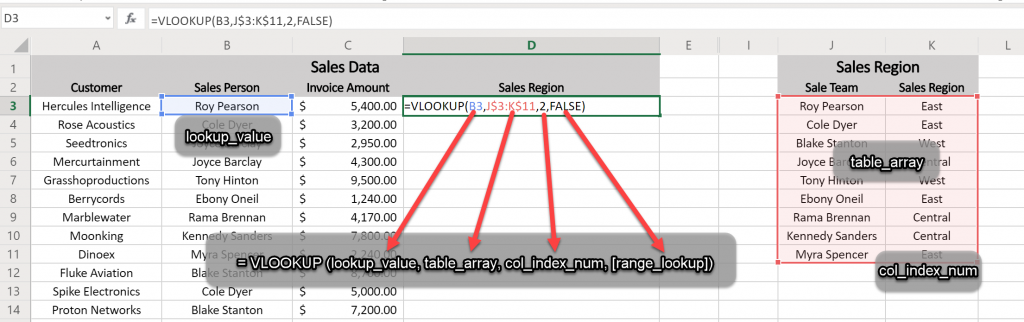
Lookup_value
The “Lookup_value” is what you are trying to categorize or assign a label to. Therefore in this example, it is the salesperson’s name.
Table_array
The “table_array” is where we are going to store the lookup or reference data. Therefore for this example, a reference table will be created with Salesperson & Region information. This can be defined using a table name reference (salesperson), a range of cells (B1:D6), or also as a range of columns (B:D).
PRO TIP – When defining a range of cells you may want to use the $ notation to create an absolute reference ($B$1:$D$6). When you go to fill down an equation this will help preserve your sanity.
Col_index_num
The “Col_index_num” tells excel which column of data should be returned from the reference data. This example is looking to determine the Region. Hence the Col_index_num is set to 2 since the Region is listed in the second column.
PRO TIP – If the lookup_value is not in the left-most column of the reference table a “LOOKUP” function may be a better alternative.
Range_lookup
The “Range_lookup” can cause unexpected results but is considered to be an optional parameter. This parameter is a True/False value in the VLOOKUP function. TRUE will find the first similar match while FALSE will only find exact matches. “True” is the default or blank value. Inaccurate data matching can happen because Excel is looking at the first similar result when using TRUE. In a list of names Excel might return the Sales Region for the first Robert on your team for all Roberts. As a result to preserve my sanity and know if there are data matching issues so I typically set it to FALSE.
WARNING – Exact match means exact, down to the number of empty spaces, punctuation, and also spelling. If you get an error or data not showing up first off try coping your lookup value into the reference table. Also, if you find hidden spaces in your data you can always useing a TRIM function to clean it up.
VLOOKUP in action
Setting up the Data
For this example, there are two tables.

- Sales Data Table – Customer Name, Salesperson, and Invoice Amount
- Sales Region – Reference table with 2 columns, salesperson’s name, and region.
Step by Step
- Start by adding a column header to the Sales Data List called “Region”
- Then add the VLOOKUP equation
- Excel Formula =vlookup(A2, Sales Rep $A$1:$B$6, 2, False)
- Cell A2 lists the salesperson’s name that we are looking for.
- Excel then looks up the name in Sales Region table and returns the region in column 2 only if the salesperson’s name matches exactly
PRO TIP – Use the fill down or quick fill to add the equation to the additional columns. Above all this is where the absolute reference ($) in the Table_Array function comes in to play. Place the cursor in the bottom right corner of the cell to fill down and double click. If there is content in the cell to the left Excel automatically adds the formula .
Tryout Excel VLOOKUP Interactive Demo Below
Try out VLOOKUP for yourself in the interactive demo sheet below.
What else can I do with Vlookup
I have used the Vlookup in a number of ways across my career to answer questions and also make informed decisions. Here is just a couple of examples to get you thinking:
- What is fiscal month or year that a transaction occurred in?
- Who is the customer that logged a support case if I only see the customer ID in the data?
- What is the text description for a group of billing codes?
Finally, for me, the lookup is just on the step in the data process. I typically use Pivot charts or graphs to analyze the data added in the lookup function. Above all learning how to use VLOOKUP in Excel has saved me hundreds of hours in manually keying and matching data.
Leave a comment below on how you use VLOOKUP in Excel.